DL / 18번째 글

ROC 곡선과 AUC: 임계값 독립적 분류 성능 평가

ROC 곡선의 TPR-FPR 트레이드오프, AUC의 확률론적 해석, PR-AUC와의 차이, 다중 클래스 확장, 최적 임계값 선택 방법을 실전 코드와 함께 완전히 이해한다.

PALDYN Team2026.04.3032 MIN READ

지난 글에서 혼동 행렬 네 칸에서 정밀도·재현율·F1까지 지표를 유도하고 읽는 법을 봤다. 그 지표들은 특정 임계값(보통 0.5)에서의 성능을 보여준다. 그런데 모델의 "진짜" 분리 능력은 임계값에 상관없이 얼마나 양성과 음성을 잘 구분하는가에 있다. ROC 곡선과 AUC는 모든 임계값에서의 성능을 하나의 곡선과 하나의 숫자로 압축한다.

이 글은 작은 예제 하나를 끝까지 들고 간다. 샘플 열 개에 점수를 매긴 뒤 곡선을 손으로 찍고, 그 면적이 왜 「양성이 음성을 이길 확률」과 같은지 쌍을 세어 확인한다. 그다음 그 숫자가 어디서 우리를 속이는지 — 극심한 불균형, 확률 보정, 클래스가 셋 이상인 경우 — 를 차례로 본다.

임계값에 묶인 지표

0.5의 자리

분류 모델은 대개 곧바로 「양성」·「음성」을 내놓지 않는다. 로지스틱 회귀든 랜덤 포레스트든 신경망이든 먼저 샘플마다 점수를 내고, 그 점수가 어떤 기준을 넘으면 양성이라고 선언한다. 이 기준이 임계값이다. 점수는 모델이 내는 연속값이고, 임계값은 그 연속값을 두 칸으로 자르는 칼이며, 혼동 행렬은 그렇게 자른 결과를 정답과 맞대어 센 표다.

predict()를 부르면 sklearn은 이진 분류에서 확률 0.5를 칼로 쓴다. 그래서 0.5가 무슨 자연 상수처럼 느껴지지만 특별한 근거는 없다. 양성과 음성이 반반이고, 두 종류의 실수가 똑같이 비싸고, 모델의 확률이 정확히 보정되어 있을 때만 0.5가 합리적인 자리다. 셋 중 하나만 어긋나도 더 나은 칼 자리가 따로 있다.

네 칸의 이동

예제를 하나 세운다. 양성 4개, 음성 6개, 모두 10개 샘플에 모델이 다음 점수를 매겼다(P는 양성, N은 음성). 점수가 높은 쪽부터 늘어놓았다.

순위	1	2	3	4	5	6	7	8	9	10
점수	0.95	0.85	0.80	0.70	0.60	0.55	0.45	0.40	0.30	0.20
정답	P	P	N	P	N	N	P	N	N	N

임계값 0.5에서 자르면 위의 여섯 개가 양성 판정이다. 그 안에 진짜 양성이 셋(TP=3), 음성이 셋(FP=3)이고, 아래 넷 중에 놓친 양성이 하나(FN=1), 제대로 거른 음성이 셋(TN=3)이다. 정밀도는 3/6=0.5, 재현율은 3/4=0.75다.

칼을 0.75로 올리면 위의 셋만 남는다. TP=2, FP=1, FN=2, TN=5가 되어 정밀도는 0.67로 오르고 재현율은 0.5로 떨어진다. 칼을 0.4로 내리면 위의 여덟이 양성이 되어 재현율은 1.0이 되지만 FP가 4로 늘어난다. 모델은 하나도 바뀌지 않았는데 네 칸이 칼 자리를 따라 계속 움직인다. 「이 모델의 정밀도는 0.5다」라는 말은 사실 「이 모델을 0.5에서 잘랐을 때의 정밀도는 0.5다」의 줄임말이다.

순위 지표

그렇다면 칼 자리와 무관한 모델의 성질은 무엇인가. 위 표를 다시 보면 칼을 어디에 두든 바뀌지 않는 것이 하나 있다 — 샘플들이 늘어선 순서다. 양성이 위쪽에 몰려 있을수록 어떤 칼을 대도 좋은 결과가 나오고, 양성과 음성이 뒤섞여 있을수록 어디를 잘라도 실수가 난다.

ROC 곡선과 AUC는 이 순서만 본다. 점수의 절댓값이 아니라 누가 누구보다 위에 있느냐만 따지므로, 점수 전체를 제곱하거나 로그를 씌우는 식으로 순서를 보존하는 변환을 해도 값이 그대로다. 이 성질이 이 지표의 강점이자, 뒤에서 볼 한계의 뿌리다.

ROC 곡선

두 축

ROC(Receiver Operating Characteristic) 곡선은 X축에 FPR(False Positive Rate), Y축에 TPR(True Positive Rate)을 놓고 임계값을 1에서 0까지 내리면서 찍히는 점들을 이은 궤적이다.

TPR = TP / (TP + FN) — 실제 양성 중 잡아낸 비율. 재현율·민감도와 같은 값이다.
FPR = FP / (FP + TN) — 실제 음성 중 잘못 양성으로 판정한 비율. 1에서 특이도를 뺀 값이다.

두 비율은 분모가 다르다는 점이 중요하다. TPR은 양성끼리만, FPR은 음성끼리만 나눈다. 그래서 두 축은 각각 한 클래스 안에서만 계산되고, 양성이 몇 개이고 음성이 몇 개인지의 비율이 곡선 모양에 직접 들어가지 않는다. 임계값을 낮추면 더 많은 것을 양성으로 선언하므로 TPR과 FPR이 함께 오르고, 높이면 함께 내려간다. 곡선은 이 둘을 맞바꾸는 비율을 한눈에 보여 준다.

한 점씩 찍기

앞의 열 개로 곡선을 직접 그려 보자. 절차는 단순하다. 점수 내림차순으로 줄을 세우고, 칼을 맨 위에서부터 한 칸씩 내린다. 칼 아래로 새로 넘어온 샘플이 양성이면 TPR이 1/4만큼 오르고(위로 한 칸), 음성이면 FPR이 1/6만큼 오른다(오른쪽으로 한 칸).

시작: 아무것도 양성이 아니다 → (0, 0)
0.95 P, 0.85 P → 위로 두 칸, (0, 0.5)
0.80 N → 오른쪽 한 칸, (1/6, 0.5)
0.70 P → 위로 한 칸, (1/6, 0.75)
0.60 N, 0.55 N → 오른쪽 두 칸, (3/6, 0.75)
0.45 P → 위로 한 칸, (3/6, 1.0)
남은 N 셋 → 오른쪽 세 칸, (1, 1)

점수 열 개로 ROC 곡선을 한 칸씩 찍는 과정

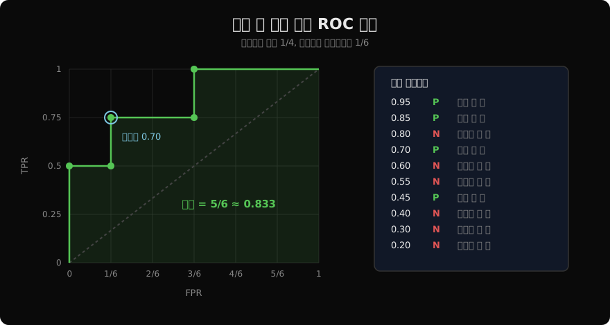
곡선 위의 한 점은 곧 하나의 임계값이다. 점 (1/6, 0.75)는 「0.70 이상을 양성으로 부르면 양성의 75%를 잡고 음성의 17%를 잘못 부른다」는 뜻이고, 실제로 배포할 때 고르는 것은 이 점들 중 하나다. 이렇게 고른 점을 운영점이라 부른다. 샘플이 많아지면 계단 한 칸이 잘게 쪼개져 매끈한 곡선처럼 보일 뿐, 원리는 이 계단 그대로다. 점수가 같은 샘플이 양성·음성 섞여 있으면 그 칸은 위와 오른쪽으로 동시에 가는 대각선이 된다.

세 모양

곡선의 모양만 봐도 모델을 읽을 수 있다.

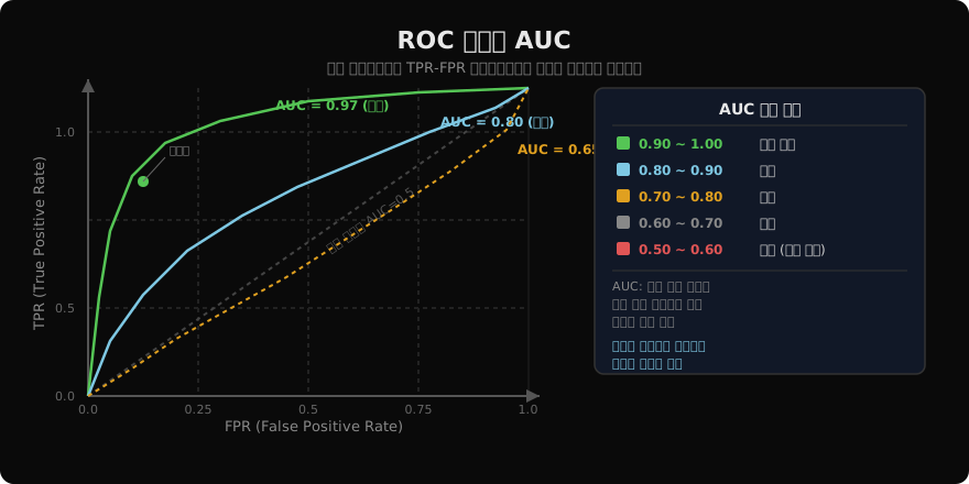
왼쪽 위 모서리 (0, 1)을 지나는 곡선은 완벽한 분리다. 칼 하나로 양성은 전부, 음성은 하나도 안 걸리는 자리가 있다는 뜻이다.
(0, 0)과 (1, 1)을 잇는 대각선은 무작위 점수다. 칼을 어디에 대든 양성과 음성이 같은 비율로 걸린다.
대각선 아래로 처지는 곡선은 순서가 뒤집힌 모델이다. 점수를 거꾸로 쓰면 오히려 쓸 만해지므로, 이런 곡선이 나오면 모델보다 라벨 인코딩이나 predict_proba의 열 순서를 먼저 의심한다.

ROC 곡선과 AUC 해석

AUC의 확률 해석

쌍 비교

AUC(Area Under the ROC Curve)는 ROC 곡선 아래의 면적으로 0에서 1 사이 값을 갖는다. 예제 계단의 면적을 구해 보자. 계단은 음성을 만날 때마다 오른쪽으로 1/6씩 가고, 그때의 높이가 그 칸의 면적을 정한다. 음성 여섯을 만날 때의 높이는 차례로 0.5, 0.75, 0.75, 1, 1, 1이므로

\text{AUC} = \frac{0.5 + 0.75 + 0.75 + 1 + 1 + 1}{6} = \frac{5}{6} \approx 0.833

이다. 이 숫자는 면적 말고 다른 방식으로도 똑같이 나온다. 양성 하나와 음성 하나를 짝지으면 쌍이 $4 \times 6 = 24$ 개 생긴다. 각 쌍에서 양성의 점수가 음성보다 높은지를 세어 보면 0.95와 0.85는 음성 여섯을 모두 이기고, 0.70은 0.80 하나에만 지고 다섯을 이기며, 0.45는 아래의 셋만 이긴다. $6 + 6 + 5 + 3 = 20$ , 곧 24쌍 중 20쌍에서 순서가 맞았고 $20/24 = 5/6$ 이다.

양성 4개와 음성 6개로 만든 24쌍 중 순서가 맞는 20쌍

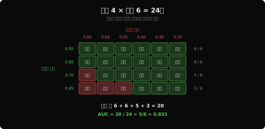
우연이 아니다. 계단에서 음성 하나를 만났을 때의 높이는 「그 음성보다 점수가 높은 양성의 비율」이고, 그것을 음성 전체에 대해 평균한 것이 면적이다. 그러니 AUC는 임의로 뽑은 양성 하나가 임의로 뽑은 음성 하나보다 높은 점수를 받을 확률이다. AUC=0.85면 그런 쌍의 85%에서 모델이 순서를 맞힌다는 뜻이고, 0.5는 동전 던지기, 1.0은 모든 쌍을 맞힌 완벽한 분리다. 점수가 똑같은 쌍은 반만 맞힌 것으로 친다.

Mann-Whitney U

통계학에는 이 쌍 세기를 이미 부르는 이름이 있다. 두 집단 중 한쪽 값이 다른 쪽보다 큰 경향이 있는지를 순위만으로 검정하는 Mann-Whitney U 검정이다. 그 검정 통계량 U가 바로 「양성이 음성을 이긴 쌍의 수」이고, 쌍의 총수로 나누면 AUC가 된다.

U는 쌍을 하나하나 비교하지 않고 순위의 합으로 빠르게 구할 수 있다. 열 개를 점수 오름차순으로 1위부터 10위까지 매기면 양성은 4위(0.45), 7위(0.70), 9위(0.85), 10위(0.95)에 있다. 양성 순위의 합을 $R_P$ , 양성 수를 $n_P$ 라 하면

U = R_P - \frac{n_P(n_P+1)}{2} = (4+7+9+10) - \frac{4 \cdot 5}{2} = 30 - 10 = 20

으로 쌍 세기와 같은 20이 나온다. 빼는 항은 양성끼리 순위를 나눠 가진 몫이다. 이 식 덕분에 AUC는 정렬 한 번, 곧 $O(n \log n)$ 에 계산되고, 샘플이 백만 개여도 쌍 1조 개를 비교할 필요가 없다.

AUC의 한계

확률 해석은 AUC가 무엇을 말하지 않는지도 정확히 알려 준다.

첫째, AUC는 운영점 하나의 성능을 말하지 않는다. 두 모델의 AUC가 같아도 곡선이 교차할 수 있다 — 한쪽은 FPR이 낮은 왼쪽 구간에서 강하고, 다른 쪽은 오른쪽 구간에서 강한 식이다. 스팸 필터처럼 FPR 1% 근처에서만 운영할 거라면 곡선 전체 면적보다 그 구간이 중요하다. sklearn의 roc_auc_score는 max_fpr 인자로 곡선 앞부분만 잘라 표준화한 부분 AUC를 준다.

둘째, AUC는 점수가 확률로 얼마나 정확한지 말하지 않는다. 순서만 보므로 모든 점수를 절반으로 줄여도 AUC는 그대로다. 이 문제는 뒤의 보정에서 다시 다룬다.

셋째, AUC는 실수의 비용을 모른다. 암을 놓치는 것과 건강한 사람을 재검사로 부르는 것의 무게가 다르다는 사실은 곡선 어디에도 들어가 있지 않다. 그 무게는 임계값을 고를 때 사람이 넣어야 한다.

두 모델을 실제 데이터에서 비교하는 기본 코드는 다음과 같다.

from sklearn.linear_model import LogisticRegression
from sklearn.ensemble import RandomForestClassifier
from sklearn.metrics import (roc_curve, roc_auc_score,
                              average_precision_score)
from sklearn.preprocessing import StandardScaler
from sklearn.pipeline import Pipeline
from sklearn.model_selection import train_test_split
from sklearn.datasets import load_breast_cancer

X, y = load_breast_cancer(return_X_y=True)
X_train, X_test, y_train, y_test = train_test_split(
    X, y, test_size=0.2, stratify=y, random_state=42)

# 두 모델 비교
models = {
    'LR':  Pipeline([('s', StandardScaler()),
                     ('m', LogisticRegression(max_iter=1000))]),
    'RF':  RandomForestClassifier(n_estimators=200, random_state=42)
}

for name, m in models.items():
    m.fit(X_train, y_train)
    y_score = m.predict_proba(X_test)[:, 1]

    auc = roc_auc_score(y_test, y_score)
    ap  = average_precision_score(y_test, y_score)
    fpr, tpr, thresholds = roc_curve(y_test, y_score)

    print(f"{name}: ROC-AUC={auc:.4f}  PR-AUC={ap:.4f}")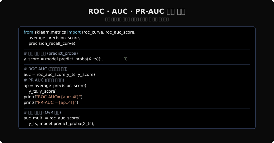

ROC AUC 코드

roc_auc_score에는 predict()가 내놓는 0/1이 아니라 predict_proba의 양성 열을 넘겨야 한다. 0/1을 넘기면 곡선에 점이 하나뿐이라 모든 임계값을 훑는다는 의미가 사라진다.

불균형과 PR 곡선

TN의 낙관

양성이 1%인 데이터를 생각해 보자. 양성 100개, 음성 9,900개다. 어떤 모델이 한 임계값에서 양성 80개를 잡고(TPR 0.8), 음성 495개를 잘못 불렀다(FPR = 495/9,900 = 0.05). ROC 곡선 위에서 (0.05, 0.8)은 왼쪽 위에 가까운 훌륭한 점이다.

그런데 이 모델이 「양성」이라고 부른 575개 중 진짜 양성은 80개뿐이다. 정밀도가 80/575, 약 0.14다. 알림을 일곱 번 받으면 여섯 번은 헛걸음이라는 뜻이다. FPR 5%가 작아 보이는 것은 분모에 TN 9,405개가 버티고 있기 때문이다. 음성이 압도적으로 많으면 FP가 수백 개로 늘어나도 FPR은 좀처럼 오르지 않고, ROC 곡선과 AUC는 계속 좋아 보인다. ROC가 클래스 비율에 흔들리지 않는다는 앞의 성질이 여기서는 오히려 현실을 가린다.

PR 기준선

이럴 때 쓰는 것이 PR 곡선이다. X축에 재현율, Y축에 정밀도를 놓고 같은 방식으로 임계값을 훑는다. 정밀도의 분모는 TP+FP, 곧 「모델이 양성이라 부른 것」이라 TN이 끼어들 자리가 없다. 곡선 아래 면적은 보통 평균 정밀도(Average Precision, AP)로 근사하는데, 양성을 하나 만날 때마다 그 자리의 정밀도를 적어 두고 평균을 낸 값이다.

예제 열 개에 적용하면 양성이 1, 2, 4, 7번째에 있으므로 그 자리의 정밀도는 1/1, 2/2, 3/4, 4/7이고 평균은 약 0.830이다. ROC-AUC 0.833과 비슷하지만, 이 예제는 양성이 40%라 불균형이 거의 없기 때문이다.

PR 곡선에서 무작위 모델이 얻는 값은 0.5가 아니라 양성 비율이다. 점수가 순서와 무관하면 어디서 자르든 잘린 무리 속 양성의 비율이 전체 비율과 같기 때문이다. 예제의 기준선은 0.4이고, 양성이 1%인 데이터의 기준선은 0.01이다. 그래서 AP=0.3은 양성 비율 40%에서는 무작위보다 못한 값이지만 1%에서는 서른 배 나은 값이다. AP는 반드시 기준선과 나란히 보고한다.

from sklearn.metrics import average_precision_score

ap = average_precision_score(y_test, y_score)
baseline = y_test.mean()   # 양성 비율 = 무작위 모델의 AP
print(f"AP={ap:.4f}  기준선={baseline:.4f}")

PR-AUC로 갈 때

두 지표는 경쟁하는 것이 아니라 다른 질문에 답한다. ROC-AUC는 「양성과 음성을 얼마나 잘 가르는가」를, PR-AUC는 「양성이라고 부른 것을 얼마나 믿을 수 있는가」를 묻는다. 양성이 대략 5%를 밑돌고, 관심이 드문 양성을 찾아내는 쪽에 있다면 — 사기 탐지, 희귀 질환 선별, 결함 검출 — PR-AUC가 실제 사용 경험에 더 가깝다. 양성과 음성이 비슷하게 섞여 있거나 두 실수가 대칭적이면 ROC-AUC로 충분하다.

한 가지 더, PR-AUC는 양성 비율에 따라 값이 바뀌므로 양성 비율이 다른 두 데이터셋의 PR-AUC를 나란히 놓고 비교하면 안 된다. 같은 모델이라도 양성이 드문 쪽에서 AP가 낮게 나온다. 반면 ROC-AUC는 그런 비교가 비교적 안전하다.

임계값 선택과 보정

Youden J와 F1

곡선을 봤으면 결국 그 위의 한 점을 골라 배포해야 한다. 가장 흔한 기준 둘이 있다.

Youden J는 $J = \text{TPR} - \text{FPR}$ 로, 대각선에서 곡선까지의 세로 거리다. 이 값이 가장 큰 점은 대각선에서 가장 멀리 떨어진 운영점이다. 예제의 꺾인 점 셋에서 J를 재면 (0, 0.5)는 0.5, (1/6, 0.75)는 약 0.583, (0.5, 1.0)은 0.5이므로 임계값 0.70이 뽑힌다.

F1 최대화는 정밀도와 재현율의 조화 평균이 가장 큰 칼 자리를 고른다. 같은 예제에서 0.85로 자르면 F1은 0.667, 0.70이면 0.75, 0.45면 약 0.727로 역시 0.70이 이긴다. 두 기준이 늘 일치하는 것은 아니다. Youden J는 TN을 보므로 음성이 많은 데이터에서 FPR을 조금 희생해 재현율을 크게 얻는 쪽으로 기울고, F1은 TN을 전혀 안 보므로 정밀도를 지키는 쪽으로 기운다.

import numpy as np
from sklearn.metrics import roc_curve, precision_recall_curve

# 방법 1: Youden's J 통계량 (TPR - FPR 최대화)
fpr, tpr, thresholds = roc_curve(y_val, val_score)
best_thr_youden = thresholds[np.argmax(tpr - fpr)]

# 방법 2: F1이 최대인 임계값
precisions, recalls, pr_thr = precision_recall_curve(y_val, val_score)
f1 = 2 * precisions * recalls / (precisions + recalls + 1e-9)
best_thr_f1 = pr_thr[np.argmax(f1[:-1])]

# 방법 3: FPR ≤ 0.05 제약 하에 TPR 최대화
ok = np.where(fpr <= 0.05)[0]
best_thr_fpr = thresholds[ok[np.argmax(tpr[ok])]]

f1[:-1]로 마지막 원소를 떼는 것은 precision_recall_curve가 정밀도·재현율 배열 끝에 임계값 없는 점 하나를 덧붙여 돌려주기 때문이다.

비용 행렬

J와 F1은 두 실수의 무게를 암묵적으로 정해 버린다. 무게를 알고 있다면 직접 넣는 편이 정직하다. 비용 행렬은 FN 하나와 FP 하나가 각각 얼마를 치르는지를 적은 표다. 사기 거래 하나를 놓치면 50만 원을 잃고, 정상 거래를 막아 고객에게 확인 전화를 거는 데 5천 원이 든다면, 임계값마다 $500{,}000 \times FN + 5{,}000 \times FP$ 를 계산해 가장 작은 칼 자리를 고른다. 이 경우 FN이 백 배 비싸므로 칼은 한참 아래로 내려간다.

위 코드의 방법 3처럼 제약 조건으로 거는 방식도 있다. 「오경보는 음성의 5%까지만 허용한다」처럼 운영 쪽이 한도를 정해 주면, 그 안에서 TPR이 가장 높은 점을 고른다. 알림을 사람이 처리해야 하는 시스템에서는 하루에 감당할 수 있는 알림 수가 곧 FPR 한도가 된다.

검증과 재조정

임계값은 학습에 쓰지 않은 검증 세트에서 고르고, 그 값을 고정한 채 테스트 세트에서 한 번 확인한다. 테스트 세트에서 곡선을 보고 가장 좋은 칼을 고른 다음 같은 테스트 세트로 성능을 보고하면, 임계값이라는 파라미터 하나를 테스트 데이터에 맞춘 셈이 되어 숫자가 부풀려진다. 위 코드가 y_val, val_score를 쓰는 이유다.

배포한 뒤에도 임계값은 고정된 값이 아니다. 입력 데이터의 분포가 바뀌거나 양성 비율이 변하면 같은 칼로 잘라도 FPR과 정밀도가 움직인다. AUC는 그대로인데 운영 지표만 나빠지는 일이 흔하므로, 운영점의 정밀도·재현율을 따로 감시하고 필요하면 최근 데이터로 칼 자리만 다시 고른다. 모델을 다시 학습하는 것보다 훨씬 싸다.

확률 보정

AUC가 순서만 본다는 성질의 반대편에 보정(calibration)이 있다. 모델이 「0.9」라고 말한 샘플을 모아 봤을 때 실제로 그중 90% 가까이가 양성이면 보정이 잘된 모델이다. 순위는 완벽한데 0.9라고 부른 것 중 60%만 양성인 모델도 얼마든지 있다. 그런 모델은 AUC가 높아도 「이 거래가 사기일 확률 90%」 같은 문장을 그대로 믿으면 안 되고, 앞의 비용 계산처럼 확률 값 자체를 곱하는 쓰임에서 틀린 답을 낸다.

보정 상태는 신뢰도 곡선으로 본다. 예측 확률을 0~~0.1, 0.1~~0.2처럼 구간으로 나누고 구간마다 평균 예측값과 실제 양성 비율을 점으로 찍는다. 점들이 대각선 위에 있으면 잘 보정된 것이다. sklearn에서는 calibration_curve가 이 점들을 준다. 숫자 하나로 요약할 때는 Brier 점수, 곧 예측 확률과 0/1 정답의 차를 제곱해 평균한 값을 쓴다. 낮을수록 좋고, 모든 샘플에 0.5를 말하는 모델은 0.25를 받는다.

보정이 틀어졌으면 모델을 다시 학습하지 않고 점수만 고쳐 쓸 수 있다. Platt 스케일링은 점수 위에 로지스틱 함수 하나를 얹어 확률로 다시 매핑하고, isotonic 회귀는 단조 증가라는 조건만 두고 계단 함수를 맞춘다. 앞쪽은 데이터가 적을 때 안정적이고, 뒤쪽은 데이터가 많을 때 더 유연하다. sklearn의 CalibratedClassifierCV가 method='sigmoid'와 method='isotonic'으로 둘을 제공한다. 두 방법 모두 점수의 순서를 거의 보존하므로 — isotonic은 동점을 만들 수 있다 — 보정 전후 AUC는 거의 그대로이고 Brier 점수만 좋아진다. 순위와 확률이 서로 다른 성질이라는 것을 가장 잘 보여 주는 장면이다.

다중 클래스 ROC-AUC

OvR과 OvO

클래스가 셋 이상이면 ROC 곡선을 한 장으로 그릴 수 없다. 이진 문제 여럿으로 쪼갠 뒤 평균을 낸다.

OvR(One-vs-Rest)은 클래스마다 「이 클래스 대 나머지 전부」의 이진 문제를 세운다. 클래스가 K개면 곡선도 K개다. 그 클래스의 확률 열을 점수로 쓰고, 나머지 클래스는 모두 음성으로 친다.
OvO(One-vs-One)는 클래스 두 개씩 짝을 지어 그 둘에 속한 샘플만으로 AUC를 구한다. 짝은 $K(K-1)/2$ 개다. 나머지 클래스가 섞여 들지 않으므로 클래스 비율의 영향을 덜 받는다.

sklearn의 roc_auc_score는 다중 클래스에서 multi_class 인자를 반드시 정해야 하며, 정하지 않으면 오류를 낸다. 또 입력은 predict_proba의 전체 행렬이어야 하고 각 행의 합이 1이어야 한다.

from sklearn.metrics import roc_auc_score

y_proba_multi = model.predict_proba(X_test)  # (n, n_classes)

auc_macro = roc_auc_score(y_test, y_proba_multi,
                           multi_class='ovr', average='macro')
auc_weighted = roc_auc_score(y_test, y_proba_multi,
                              multi_class='ovr', average='weighted')
auc_ovo = roc_auc_score(y_test, y_proba_multi,
                         multi_class='ovo', average='macro')

macro와 weighted

K개의 AUC를 하나로 합치는 방법이 평균 방식이다. macro 평균은 클래스마다 같은 무게를 주고, weighted 평균은 클래스의 샘플 수에 비례한 무게를 준다. 샘플 900개인 클래스 A의 AUC가 0.98이고 100개인 클래스 B가 0.70이면 macro는 0.84, weighted는 $0.9 \times 0.98 + 0.1 \times 0.70 = 0.952$ 다.

어느 쪽이 맞는지는 질문에 달렸다. 드문 클래스도 똑같이 중요하다면 macro를 본다. weighted는 큰 클래스가 가려 버린 약점을 숫자에서 지워 버리기 쉽다 — 위 예에서 0.952만 보고서에 적으면 B가 거의 무작위에 가깝다는 사실이 사라진다.

클래스별 확인

그래서 평균 하나로 끝내지 말고 OvR AUC를 클래스별로 나란히 적어 두는 습관이 좋다. sklearn 버전에 따라 average=None이 클래스별 값을 돌려주기도 하지만, 가장 확실한 방법은 클래스마다 y_test == k를 정답으로, y_proba_multi[:, k]를 점수로 넣어 이진 AUC를 따로 구하는 것이다. 어떤 클래스가 다른 어떤 클래스와 헷갈리는지까지 알고 싶다면 OvO 짝별 AUC나 혼동 행렬로 내려가야 한다. 평균은 요약일 뿐이고, 고칠 곳을 알려 주는 것은 쪼개 본 숫자다.

지표 고르기

상황별 지표

지금까지 본 것을 한 표로 묶으면 다음과 같다.

상황	권장 지표
클래스 균형, 임계값 고정	F1, 정확도
임계값이 아직 정해지지 않음	ROC-AUC
양성 비율 5% 미만, 양성 찾기가 목적	PR-AUC (평균 정밀도)
실수 비용이 비대칭	비용 최소화 임계값, FPR 제약
확률 값을 그대로 씀	Brier 점수, 신뢰도 곡선
다중 클래스	macro ROC-AUC + 클래스별 AUC

보고 방식

모델 비교 단계에서는 ROC-AUC나 PR-AUC처럼 임계값과 무관한 숫자로 후보를 추리고, 배포 단계에서는 고른 운영점의 정밀도·재현율·FPR을 적는다. 둘은 서로를 대신하지 못한다. AUC 0.95짜리 모델도 칼을 잘못 대면 쓸모가 없고, 좋은 운영점 하나가 곡선 전체의 품질을 보장하지도 않는다.

보고서에는 적어도 세 가지를 함께 적어 두자. 무엇을 기준으로 임계값을 골랐는지, 그 임계값을 어느 데이터에서 골랐는지, 양성 비율이 얼마였는지다. 이 셋이 빠진 AUC와 F1은 다른 사람이 재현하거나 비교할 수 없다. 여기까지가 분류 모델을 평가하는 도구 상자이고, 다음 글에서는 출력이 범주가 아니라 연속적인 수인 회귀 모델의 평가 지표 — MAE·MSE·RMSE·R² — 로 넘어간다.

읽어주셔서 감사합니다. 😊